Documentation Index
Fetch the complete documentation index at: https://docs.sectors.app/llms.txt
Use this file to discover all available pages before exploring further.
Exploratory Data Analysis (EDA) is an essential first step in understanding stock price data, offering insights into patterns and trends over time. Stock prices represent a dynamic time series, capturing how market conditions and external events impact valuation. This article explores key EDA techniques to interpret stock price variations, from identifying patterns and anomalies to examining price changes in response to significant events, going further beyond simple moving averages from the previous recipes to uncover deeper insights.
Seasonal Decompose
Seasonal decomposition is a powerful method for breaking down stock price data into its fundamental components, revealing underlying patterns that may not be immediately visible. The technique divides the time series data into three main components:
-
Trend: This component captures the long-term movement in the data, showing the general direction (upward, downward, or stable) in stock prices over time. The trend can highlight market sentiment and provide insights into sustained patterns that might be associated with company performance or broader economic indicators.
-
Seasonal: The seasonal component reflects recurring fluctuations or cycles in the data, often influenced by periodic events like earnings announcements, fiscal quarters, or even broader economic cycles. Analyzing seasonality allows us to understand recurring behaviors in stock price movements and anticipate potential cyclic trends.
-
Residual: Also known as the “remainder” or “noise,” this component captures random fluctuations and irregularities in the data that aren’t explained by trend or seasonality. These variations can result from unexpected events, news releases, or other market anomalies.
Additive vs. Multiplicative Decomposition
When performing seasonal decomposition, it’s essential to understand the distinction between additive and multiplicative models. These two models define how the components (trend, seasonal, and residual) interact within the time series data.
-
Additive Model: In an additive model, the components are added together to reconstruct the original time series. This model assumes that the effect of each component is constant over time. It’s most suitable when variations in seasonality and residuals are relatively uniform.
- Formula:
Y(t) = Trend(t) + Seasonal(t) + Residual(t)
-
Multiplicative Model: In a multiplicative model, the components are multiplied to recreate the time series. This model is typically used when the seasonal variations or noise increase or decrease proportionally with the level of the trend. This approach is effective when the amplitude of seasonal effects grows with stock price changes.
- Formula:
Y(t) = Trend(t) * Seasonal(t) * Residual(t)
Choosing between these models depends on the nature of the stock price data. An additive model suits data with relatively stable seasonality, while a multiplicative model is preferable if seasonality varies with the level of the data.
Code Implementation
Here’s how we can put this into practice. Below is a code snippet to retrieve stock market data from August 2019 up to the current date for BBCA. Get ready—we’re about to dive into an exciting journey of exploration and analysis!
import requests
import time
from datetime import datetime, timedelta
from google.colab import userdata
api_key = userdata.get('SECTORS_API_KEY')

ticker = "BBCA"

url = f"https://api.sectors.app/v2/daily/{ticker}/"

headers = {"Authorization": api_key}

# today
end_date = time.strftime("%Y-%m-%d")
#start date: end_date - 90 days
start_date = (datetime.strptime(end_date, "%Y-%m-%d") - timedelta(days=90)).strftime("%Y-%m-%d")

# accumulator array
data = []


def execute(i : int): # recursive procedure
    global start_date, end_date, data
    params = {
    "start": start_date,
    "end": end_date,
    }
    response = requests.request("GET", url, headers=headers, params=params)

    if response.status_code == 200:
        res = response.json()
        # concatenate
        # reverse res
        res = res[::-1]
        data = data + res
    else:
        print(f"Request failed with status code {response.status_code}")


    if(i == 0) : return

    else :
        end_date =  (datetime.strptime(start_date, "%Y-%m-%d") - timedelta(days=1)).strftime("%Y-%m-%d")
        start_date = (datetime.strptime(end_date, "%Y-%m-%d") - timedelta(days=90)).strftime("%Y-%m-%d")

        return execute(i-1)

# try to fulfill with 20 iterations
execute(20)
# reverse the order
df = pd.DataFrame(data[::-1])
data variable :
| symbol | date | close | volume | market_cap |
|---|
| BBCA.JK | 2019-08-12 | 6040 | 52705000 | NaN |
| BBCA.JK | 2019-08-13 | 6015 | 84406000 | NaN |
| BBCA.JK | 2019-08-14 | 6010 | 81942000 | NaN |
| BBCA.JK | 2019-08-15 | 6000 | 52561500 | NaN |
| BBCA.JK | 2019-08-16 | 5960 | 49821500 | NaN |
seasonal_decompose from statsmodel
from statsmodels.tsa.seasonal import seasonal_decompose
df_decompose = df[["date", "close"]]
df_decompose["date"] = pd.to_datetime(df_decompose["date"])
df_decompose.set_index("date", inplace=True)
result = seasonal_decompose(df_decompose['close'], model='additive', period=365)
fig = result.plot()
fig.show()
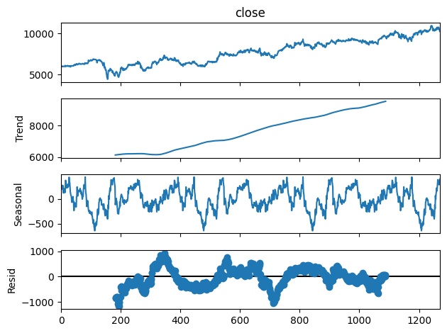 With the seasonal decomposition complete, we can now analyze the periods when the seasonal trend reaches its minimum and maximum values. This helps us understand the cyclical behavior of the stock price over time.
Using the
With the seasonal decomposition complete, we can now analyze the periods when the seasonal trend reaches its minimum and maximum values. This helps us understand the cyclical behavior of the stock price over time.
Using the seasonal component, we identify the dates where these minimum and maximum values occur. Below is the code snippet to accomplish this:
import calendar

# Store the seasonal component in a DataFrame
seasonal = result.seasonal

# Find the date where the seasonal component has minimum and maximum values
idx_min_date = seasonal.idxmin()
idx_max_date = seasonal.idxmax()
min_value = seasonal.min()
max_value = seasonal.max()

# Retrieve the min_date and max_date from df_decompose based on the index
min_date = df_decompose.loc[idx_min_date, 'date']
max_date = df_decompose.loc[idx_max_date, 'date']

# Print the minimum and maximum period of the seasonal trend
print(f"Minimum period of the seasonal trend: {calendar.month_name[min_date.month]} {min_date.day}")
print(f"Maximum period of the seasonal trend: {calendar.month_name[max_date.month]} {max_date.day}")
Explanation:
-
Extract the Seasonal Component: We store the seasonal component from the
seasonal_decompose result in a variable called seasonal.
-
Find Min/Max Values: We use
.idxmin() and .idxmax() to get the dates where the seasonal trend reaches its minimum and maximum values, respectively.
-
Map Month Numbers to Names: Using Python’s
calendar.month_name, we convert the month numbers of these dates into their corresponding month names.
-
Display the Results: We print the minimum and maximum period of the seasonal trend, showing the month and day for each.
The output will look like this:
Minimum period of the seasonal trend: January-22
Maximum period of the seasonal trend: December-3
Market Volatility
Market volatility refers to the speed and extent of price changes for a financial instrument over a given time period. High volatility suggests significant price swings, whereas low volatility indicates smaller changes.
Common ways to measure volatility include historical volatility and implied volatility, the latter being calculated from options prices.
To better understand market volatility, we can analyze the daily returns of the stock as the first step.
Daily return represents the percentage change in stock price from one day to the next, which helps in visualizing the frequency and scale of price fluctuations.
Using the code below, we calculate daily returns and create a time series plot to observe these variations over time:
import plotly.express as px

# Calculate daily returns as a percentage
df_return = pd.DataFrame(df['close'])
df_return['daily_return'] = df_return['close'].pct_change() * 100
df_return['date'] = df['date']
df_return.dropna(inplace=True)

# Plot the time series of daily return percentage
fig = px.line(df_return, x='date', y='daily_return',
              color_discrete_sequence=['red'],
              labels={'value': 'Daily Return', 'variable': 'Legend'},
              title='Daily Return of the Companies')
fig.show()
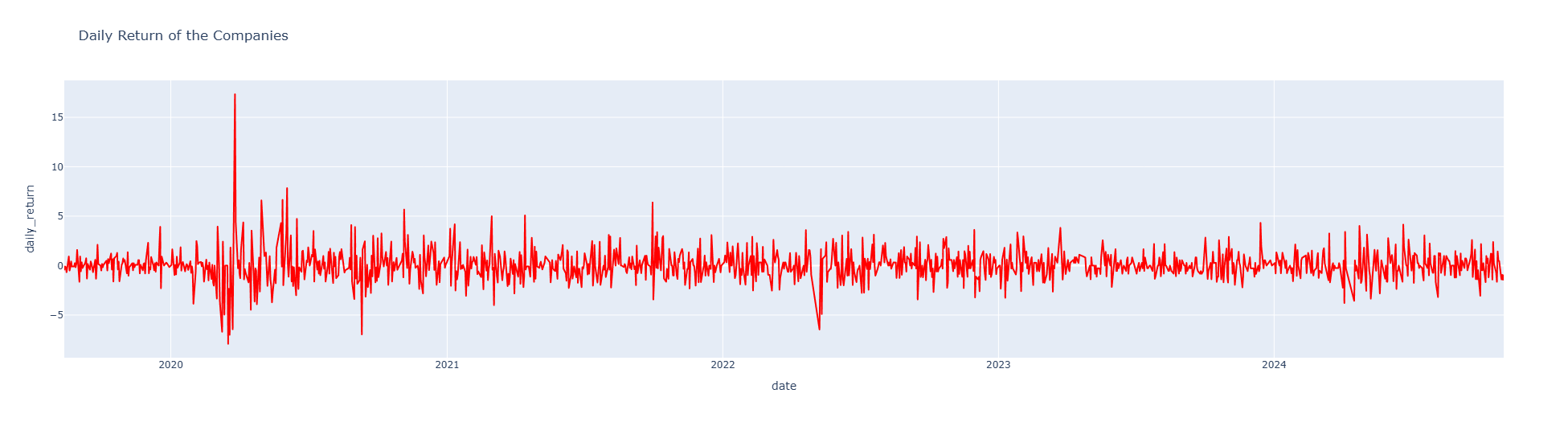 The resulting plot shows the daily return percentage, highlighting periods of high and low volatility.
Sharp peaks indicate days with significant price changes, signaling higher volatility, while flatter areas reflect more stable, low-volatility periods.
After that, we could see the distribution of daily return using this code below.
The resulting plot shows the daily return percentage, highlighting periods of high and low volatility.
Sharp peaks indicate days with significant price changes, signaling higher volatility, while flatter areas reflect more stable, low-volatility periods.
After that, we could see the distribution of daily return using this code below.
fig_hist = px.histogram(df_return, x='daily_return', nbins=30,
                        title='Distribution of Daily Return',
                        labels={'daily_return': 'Daily Return (%)'})
fig_hist.show()
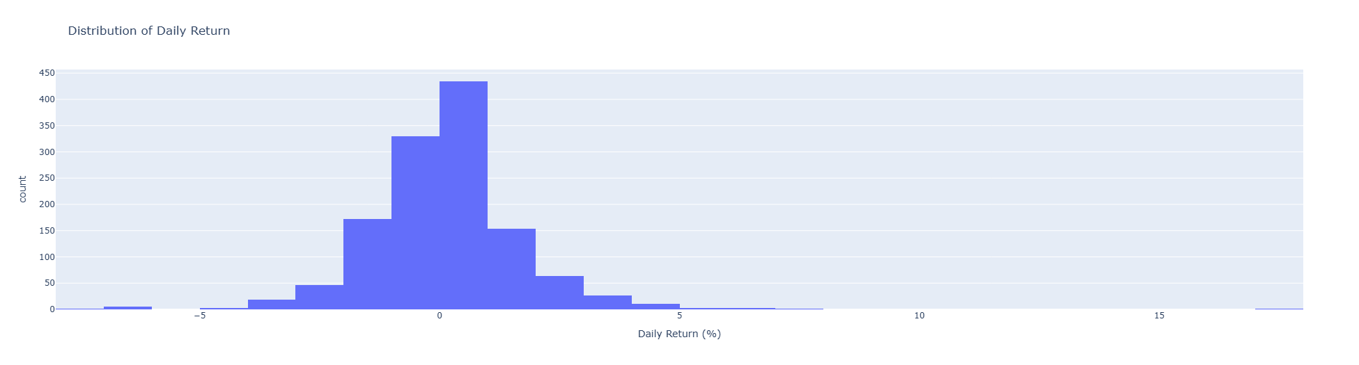 From the histogram above, we can infer that >50% data have positive daily return.
The Annualized Volatility
To gain further insights into market volatility, we can calculate the annualized volatility of the stock. Annualized volatility provides an estimate of the stock’s price fluctuation over a year and helps investors understand long-term risk.
Using a 21-day rolling window (approximately one trading month), we compute the daily standard deviation of returns and scale it to an annual measure by multiplying by the square root of 252, the typical number of trading days in a year. The code below demonstrates this calculation and visualization:
import numpy as np

# Define rolling window for calculating volatility
window = 21

# Calculate rolling annualized volatility
df_decompose['volatility'] = (df_decompose['close'].pct_change().rolling(window=window).std() * np.sqrt(252)).reset_index(0, drop=True)
df_decompose.dropna(inplace=True)
# Plot the time series of annualized volatility
fig = px.line(df_decompose, x='date', y='volatility',
              color_discrete_sequence=['green'],
              labels={'value': 'Volatility', 'variable': 'Legend'},
              title='Volatility of the Companies')
fig.show()
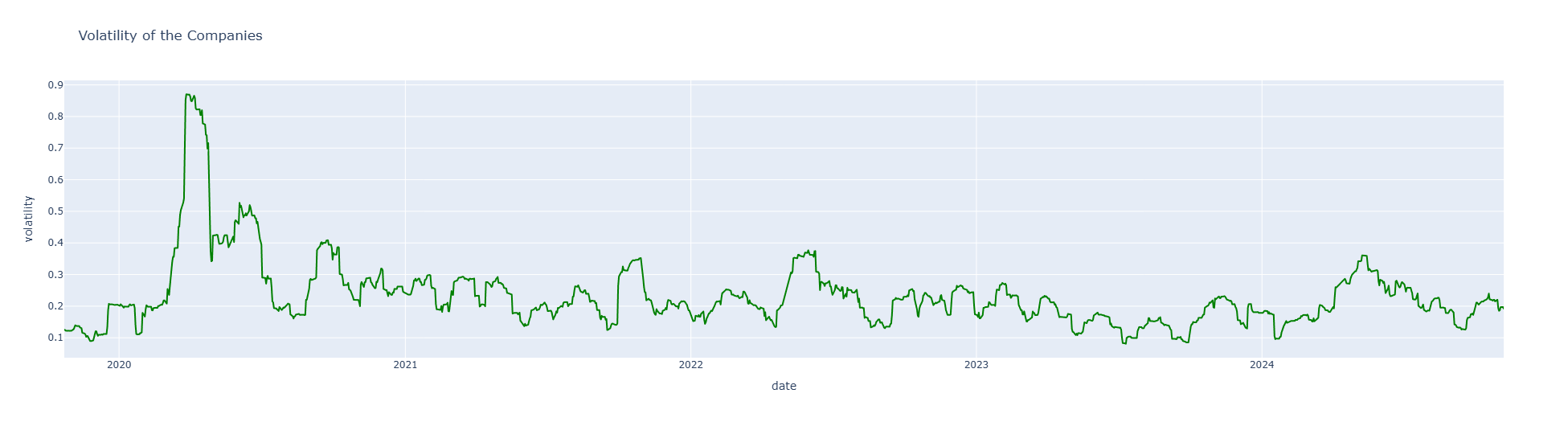 The plot above visualizes the annualized volatility of the stock over time, where spikes indicate periods of increased volatility and thus higher risk.
This rolling measure of volatility allows investors to observe how risk levels change over different timeframes and make more informed decisions regarding entry and exit points in response to market conditions.
The plot above visualizes the annualized volatility of the stock over time, where spikes indicate periods of increased volatility and thus higher risk.
This rolling measure of volatility allows investors to observe how risk levels change over different timeframes and make more informed decisions regarding entry and exit points in response to market conditions.
Forecasting the Volatility using Machine Learning
After we get the annualized volatility, we could perform the machine learning method in order to forecast the future volatility
1. Feature Engineering
In preparation for forecasting volatility, we perform feature engineering to create relevant indicators that capture different aspects of stock behavior.
These features provide valuable insights into trends, momentum, and volume, which can influence volatility.
- 21-Day Moving Average: A rolling mean over the past 21 days, which smooths price data to highlight longer-term trends.
- Relative Strength Index (RSI): A momentum indicator over a 14-day window that ranges from 0 to 100, indicating overbought or oversold conditions.
- On-Balance Volume (OBV): A volume-based indicator that reflects buying and selling pressure to reveal whether volume is moving in or out of the stock.
- Moving Average Convergence Divergence (MACD): A trend-following measure of the difference between two moving averages, helping detect shifts in price trends.
These engineered features provide insights into stock behavior and prepare the data for machine learning.
The code below generates these features and removes any missing values:
from ta.momentum import RSIIndicator
from ta.trend import MACD
from ta.volume import OnBalanceVolumeIndicator

# Feature: 21-day Moving Average
df_decompose['MA_21'] = df_decompose['close'].rolling(window=21).mean()

# Feature: RSI
rsi = RSIIndicator(df_decompose['close'], window=14)
df_decompose['RSI'] = rsi.rsi()

# Feature : On-Balance Volume (OBV)
obv = OnBalanceVolumeIndicator(df['close'], df['volume'])
df_decompose['OBV'] = obv.on_balance_volume()

# Feature: MACD
macd = MACD(df_decompose['close'])
df_decompose['MACD'] = macd.macd_diff()

# Drop NaN values
df_decompose.dropna(inplace=True)
2. Modeling with Random Forest Regressor
With the features now engineered, we can proceed to building a machine learning model to forecast future volatility.
In this example, we use a Random Forest Regressor to predict the stock’s future volatility based on the feature set we’ve created.
Random Forests are effective for this type of problem because they handle complex patterns in the data well and are generally robust without requiring extensive parameter tuning.
The code below implements this entire pipeline:
from sklearn.model_selection import train_test_split
from sklearn.ensemble import RandomForestRegressor
from sklearn.metrics import mean_squared_error
import numpy as np

# Create target variable
df_decompose['future_volatility'] = df_decompose['volatility'].shift(-21)  # Forecast 21 days ahead

# Drop NaN values
df_decompose.dropna(inplace=True)

# Features and target
X = df_decompose[['MA_21', 'RSI', 'OBV', 'MACD', 'volatility']]
y = df_decompose['future_volatility']

# Split data into training and testing sets
X_train, X_test, y_train, y_test = train_test_split(X, y, test_size=0.2, random_state=42)

# Train Random Forest model
model = RandomForestRegressor(n_estimators=100, random_state=42)
model.fit(X_train, y_train)

# Predict on test data
y_pred = model.predict(X_test)

# Calculate RMSE
rmse = np.sqrt(mean_squared_error(y_test, y_pred))
print(f'Root Mean Squared Error: {rmse}')
Root Mean Squared Error: 0.05083765007739254
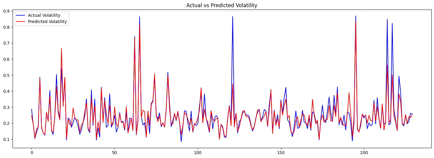
3. Evaluating the Model
To evaluate the effectiveness of our volatility forecasting model, we can visually compare the actual and predicted volatility values on the test set.
This helps us understand how well the model captures the volatility patterns over time.
The plot below shows the actual and predicted values side-by-side:
import matplotlib.pyplot as plt

# Plot the actual and predicted volatility values
plt.figure(figsize=(18, 6))
plt.plot(y_test.values, label='Actual Volatility', color='blue')
plt.plot(y_pred, label='Predicted Volatility', color='red')
plt.title('Actual vs Predicted Volatility')
plt.legend()
plt.show()
4. Incorporating Volatility Forecasting into a Stock Trading Strategy
To incorporate volatility forecasting into a trading strategy through position sizing, we can use the model’s volatility forecast to adjust the size of our trades.
A common approach is to reduce position size when higher volatility is predicted (to minimize risk) and increase position size when volatility is lower.
Here’s an example of how this concept can be implemented in Python:
-
Position Sizing Formula: We can use a basic position sizing rule where position size is inversely related to forecasted volatility. For instance:
Position Size = Target Risk / Forecasted Volatility
where Target Risk is a predefined amount of capital at risk per trade.
-
Setting Up Parameters: We define a risk factor and calculate position sizes based on forecasted volatility.
-
Implementation: Below, we calculate position sizes for each day based on the model’s volatility forecast.
import numpy as np

# Define target risk (the rupiah amount or percentage of capital to risk per trade)
target_risk = 10000  # e.g., Rp10.000 risk per trade

# Calculate position sizes based on forecasted volatility
df_decompose['position_size'] = target_risk / df_decompose['future_volatility']

# Limit position size to avoid excessively large trades during low volatility
max_position_size = 50000  # Maximum units to trade, based on strategy limits
df_decompose['position_size'] = np.minimum(df_decompose['position_size'], max_position_size)

# Example output to see the calculated position sizes
df_decompose[['date', 'future_volatility', 'position_size']].tail()
- Higher Forecasted Volatility → Smaller position sizes to limit potential losses.
- Lower Forecasted Volatility → Larger position sizes to take advantage of stable market conditions.
From the volatility forecast of BBCA stock, we can evaluate the potential position sizes for future trades.
The results are shown below:
| Date | Future Volatility | Position Size |
|---|
| 2024-08-30 | 0.211042 | 47383.833926 |
| 2024-09-02 | 0.211006 | 47392.010809 |
| 2024-09-03 | 0.208473 | 47967.750053 |
| 2024-09-04 | 0.204720 | 48847.234923 |
| 2024-09-05 | 0.212859 | 46979.355676 |