Quick Introduction
This tutorial is a supplementary resource for the workshop “Stock Portfolio Optimization with Python” using the Sectors API. It covers these topics: stock investment background and understanding the Sectors API, stock selection overview and two stock portfolio optimization models, followed by further recommendations and insights.Sectors API & Stock Investment Overview
When considering stock investments, individual investors typically focus on key questions such as: Which stocks to buy? How many shares? What’s the price, growth potential, and risk? Using the Sectors API, investors gain access to valuable data from the “Companies by Index” and “Daily Transaction Data” endpoints, including stock indexes, dates, closing prices, volumes, and market capitalizations. Next, the “Company Report” API provides additional insights such as EPS, dividends, growth metrics, and other relevant financial information. In Data Collection from Sectors API, we will explore how to effectively query this data from the API to build a portfolio optimization model. However, before diving into optimization, it’s crucial to understand the available stock indexes and their respective investment purposes.| index | Index | Focus | Investment Use |
|---|---|---|---|
| 0 | FTSE | Globally recognized index of large-cap companies | For investors seeking to track global or broad market performance |
| 1 | IDX30 | Top 30 stocks by market cap and liquidity | Suitable for blue-chip stock investors looking for stable and liquid companies |
| 2 | IDXBUMN20 | Top 20 government-owned enterprises (BUMN) | For exposure to state-owned enterprises (SOEs) benefiting from government policies |
| 3 | IDXESGL | Stocks meeting ESG (environmental, social, governance) standards | Ideal for socially responsible investors focused on sustainability and ethical investing |
| 4 | IDXG30 | Large-cap, high liquidity growth stocks | For growth-oriented investors looking for long-term capital appreciation |
| 5 | IDXHIDIV20 | 20 stocks with high dividend yields | Attractive to income-seeking investors focused on dividend income |
| 6 | IDXQ30 | Focus on quality stocks based on financial metrics | Suitable for long-term investors seeking companies with strong fundamentals |
| 7 | IDXV30 | Focus on value stocks trading below intrinsic value | Ideal for value investors looking for undervalued stocks |
| 8 | JII70 | 70 stocks complying with Shariah (Islamic law) | Suitable for Shariah-compliant investors following Islamic investment principles |
| 9 | KOMPAS100 | 100 most liquid, actively traded stocks | For investors seeking diversified exposure to Indonesia’s liquid stocks |
| 10 | LQ45 | Top 45 most liquid stocks with large market caps | Blue-chip focused, for investors looking for stability and long-term growth potential |
| 11 | SMInfra18 | 18 infrastructure-related stocks | For investors bullish on infrastructure growth and development projects in Indonesia |
| 12 | SRIKEHA18 | Tracks sustainability and social responsibility | Ideal for ESG investors prioritizing sustainable business practices |
| 13 | SRIKEHATI | Sustainability and ethical investing | Same as SRIKEHA18, for socially responsible investors |
Where to start?
Recommendation: Match your investment goals with the property of stock index.| index | Criteria | Description | Persona | Recommended Index |
|---|---|---|---|---|
| 0 | Liquidity & Stability | Investors looking for highly liquid and stable stocks that are less volatile. | Maria, a risk-averse retiree seeking low volatility and stable returns. | IDX30, LQ45, KOMPAS100 |
| 1 | Government-Owned Enterprises | For investors interested in companies benefiting from government backing and policies. | Adi, a public sector enthusiast who trusts government-driven initiatives. | IDXBUMN20 |
| 2 | Dividend Focus | Ideal for those seeking regular income from dividends. | Siti, a conservative investor who prefers stable income from dividends. | IDXHIDIV20 |
| 3 | Growth-Oriented | Suitable for long-term investors focusing on capital appreciation. | Kevin, a young professional aiming for long-term wealth through capital growth. | IDXG30 |
| 4 | Value Stocks | Investors seeking undervalued stocks trading below intrinsic value. | Tom, a value investor who looks for bargain stocks below intrinsic value. | IDXV30 |
| 5 | High-Quality Financials | Focus on stocks with strong fundamentals and good financial health. | Dewi, a financial analyst who invests in companies with strong fundamentals. | IDXQ30 |
| 6 | Shariah-Compliant Investments | For investors following Islamic principles. | Ahmad, a devout Muslim who prioritizes Shariah-compliant investments. | JII70 |
| 7 | Socially Responsible Investments | Investors interested in ESG (environmental, social, governance) and ethical business practices. | Sarah, an environmentally conscious investor focusing on ethical companies. | IDXESGL, SRIKEHA18, SRIKEHATI |
| 8 | Infrastructure Focus | For investors bullish on Indonesia’s infrastructure growth. | Indra, an infrastructure expert optimistic about Indonesia’s construction growth. | SMINFA18 |
| 9 | Broad Market Exposure | For investors wanting diversified exposure across large segments of the market. | Emily, a diversified investor looking for broad market exposure and lower risk. | FTSE, KOMPAS100 |
- Government infrastructure spending: Announcements of new airports and highways as public projects.
- Interest Rate policies: Indonesia’s central bank lowers interest rates.
- Commodity prices: Steel and cement prices drop due to global supply chain restructuring.
- Foreign Direct investment: China increases investment in Indonesia’s high-speed rail projects.
Data Collection from Sectors API
1. Stock Price Information
2. Company Report Information
Which Stock to choose?
1. Data Preprocessing
How to select stocks? For our client Indra, who’s focused on stocks from the SMInfra18 index and doesn’t want to invest in the ente it’s time to carefully select the right stocks. Several key economic factors should guide stock selection from an index:- Diversification by Industry and Sector: Ensuring exposure across different sectors to reduce risk.
- Diversification by Correlation and Returns: Selecting stocks that offer varied returns and are not too closely correlated.
- Company Growth and Dividend Information: Choosing companies with strong growth potential and reliable dividend payouts.
| date | ADHI.JK | AKRA.JK | BBNI.JK | BBRI.JK | BMRI.JK | EXCL.JK | INTP.JK | ISAT.JK | JSMR.JK | MEDC.JK | PGAS.JK | PTPP.JK | SMGR.JK | SSIA.JK | TBIG.JK | TLKM.JK | TOWR.JK | UNTR.JK |
|---|---|---|---|---|---|---|---|---|---|---|---|---|---|---|---|---|---|---|
| 2024-07-10 00:00:00 | 250.0 | 1510.0 | 4820.0 | 4850.0 | 6375.0 | 2270.0 | 7325.0 | 11000.0 | 5125.0 | 1340.0 | 1520.0 | 392.0 | 4050.0 | 1070.0 | 1935.0 | 3160.0 | 780.0 | 23550.0 |
| 2024-07-11 00:00:00 | 248.0 | 1505.0 | 4870.0 | 4840.0 | 6400.0 | 2270.0 | 7400.0 | 11500.0 | 5300.0 | 1330.0 | 1560.0 | 388.0 | 4010.0 | 1110.0 | 1990.0 | 3180.0 | 785.0 | 23500.0 |
| 2024-07-12 00:00:00 | 262.0 | 1500.0 | 5025.0 | 4900.0 | 6425.0 | 2280.0 | 7500.0 | 11400.0 | 5375.0 | 1315.0 | 1580.0 | 416.0 | 4090.0 | 1095.0 | 2000.0 | 3220.0 | 810.0 | 23500.0 |
| 2024-07-15 00:00:00 | 256.0 | 1505.0 | 5025.0 | 4820.0 | 6350.0 | 2240.0 | 7375.0 | 11425.0 | 5300.0 | 1285.0 | 1580.0 | 406.0 | 4060.0 | 1100.0 | 1970.0 | 3160.0 | 800.0 | 23750.0 |
| 2024-07-16 00:00:00 | 248.0 | 1505.0 | 4980.0 | 4730.0 | 6350.0 | 2240.0 | 7350.0 | 11650.0 | 5325.0 | 1295.0 | 1610.0 | 398.0 | 4060.0 | 1070.0 | 2010.0 | 3100.0 | 790.0 | 23800.0 |
| index | symbol | company_name | industry | sub_industry | sector | eps_estimate | revenue_estimate | eps_growth | revenue_growth | total_dividends | avg_yield_dividends |
|---|---|---|---|---|---|---|---|---|---|---|---|
| 0 | ADHI.JK | PT Adhi Karya (Persero) Tbk. | Heavy Constructions & Civil Engineering | Heavy Constructions & Civil Engineering | Infrastructures | 0.0 | 15655500000000 | -1.0 | -0.220071482804073 | 17.0694 | 0.00909244380891323 |
| 1 | AKRA.JK | PT AKR Corporindo Tbk. | Oil & Gas | Oil & Gas Storage & Distribution | Energy | 158.97 | 45464400000000 | 0.128497644987348 | 0.080249278422712 | 125.0 | 0.0483752990141511 |
| 2 | BBNI.JK | PT Bank Negara Indonesia (Persero) Tbk | Banks | Banks | Financials | 679.11 | 71617800000000 | 0.210047774618842 | 0.162937331535753 | 280.495 | 0.0517167726531625 |
| 3 | BBRI.JK | PT Bank Rakyat Indonesia (Persero) Tbk | Banks | Banks | Financials | 451.37 | 213801000000000 | 0.133420504682536 | 0.284275264842541 | 319.0 | 0.0377051925286651 |
| 4 | BMRI.JK | PT Bank Mandiri (Persero) Tbk | Banks | Banks | Financials | 657.58 | 161727000000000 | 0.114676156918109 | 0.312340707462218 | 353.958 | 0.043529000878334 |
| 5 | EXCL.JK | PT XL Axiata Tbk | Wireless Telecommunication Services | Wireless Telecommunication Services | Infrastructures | 163.4 | 36726100000000 | 0.680381983628672 | 0.136234153566179 | 42.0 | 0.011895396001637 |
| 6 | INTP.JK | Indocement Tunggal Prakarsa Tbk | Construction Materials | Construction Materials | Basic Materials | 520.15 | 19834300000000 | -0.0849079498610495 | 0.104989950838329 | 160.0 | 0.0379668477922678 |
| 7 | ISAT.JK | PT Indosat Tbk | Wireless Telecommunication Services | Wireless Telecommunication Services | Infrastructures | 804.29 | 58606500000000 | 0.439008013491739 | 0.144015096825843 | 255.7 | 0.0401271820068359 |
| 8 | JSMR.JK | PT Jasa Marga Tbk | Transport Infrastructure Operator | Highways & Railtracks | Infrastructures | 412.83 | 18012300000000 | -0.558954239095396 | -0.155090119639629 | 75.6939 | 0.00636524613946676 |
| 9 | MEDC.JK | PT Medco Energi Internasional Tbk | Oil & Gas | Oil & Gas Production & Refinery | Energy | 0.0 | 0 | 0.0 | 0.0 | 38.7888 | 0.0164257543161511 |
| 10 | PGAS.JK | PT Perusahaan Gas Negara Tbk. | Oil & Gas | Oil & Gas Storage & Distribution | Energy | 211.6 | 58229200000000 | 0.190791463560484 | 0.0309451120764361 | 141.054 | 0.0477137375622988 |
| 11 | PTPP.JK | PP (Persero) Tbk | Heavy Constructions & Civil Engineering | Heavy Constructions & Civil Engineering | Infrastructures | 0.0 | 25903000000000 | -1.0 | 0.295543484289943 | 33.842 | 0.0114528350532055 |
| 12 | SMGR.JK | Semen Indonesia (Persero) Tbk | Construction Materials | Construction Materials | Basic Materials | 390.38 | 41187700000000 | 0.214314626055841 | 0.0656209768556656 | 245.19 | 0.0204733341000974 |
| 13 | SSIA.JK | PT Surya Semesta Internusa Tbk | Heavy Constructions & Civil Engineering | Heavy Constructions & Civil Engineering | Infrastructures | 94.98 | 5564360000000 | 1.44788190848669 | 0.226263662186343 | 5.0 | 0.00422613676637411 |
| 14 | TBIG.JK | PT Tower Bersama Infrastructure Tbk | Wireless Telecommunication Services | Wireless Telecommunication Services | Infrastructures | 75.72 | 7076440000000 | NaN | 0.0656254023517294 | 60.3455 | 0.0212685994803905 |
| 15 | TLKM.JK | PT Telkom Indonesia (Persero) Tbk | Telecommunication Service | Integrated Telecommunication Service | Infrastructures | 281.35 | 161171000000000 | 0.140997881239521 | 0.0801187540210165 | 167.599 | 0.037667010165751 |
| 16 | TOWR.JK | Sarana Menara Nusantara Tbk | Wireless Telecommunication Services | Wireless Telecommunication Services | Infrastructures | 71.69 | 12786000000000 | NaN | 0.0890650998756851 | 24.1 | 0.0254231836646795 |
| 17 | UNTR.JK | United Tractors Tbk | Machinery | Construction Machinery & Heavy Vehicles | Industrials | 4274.33 | 116960000000000 | NaN | -0.0903948432978027 | 1569.0 | 0.0932280221953988 |
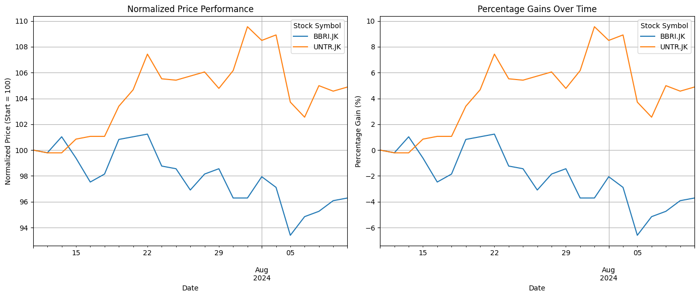
2. Exploratory Data Analysis (EDA)
Our goal is to select two or three stocks from a list of 18 for Indra to invest in. At the beginning of this section, we outlined three strategies:- Diversification by Industry and Sector: Conduct an overview analysis to understand the information better.
- Diversification by Correlation: Examine the correlation matrix based on stock price evolution.
- Company Growth and Dividend Information: Extract all relevant information beyond sector and industry, normalize the data, and assign a score to each stock.
| industry | count |
|---|---|
| Wireless Telecommunication Services | 4 |
| Heavy Constructions & Civil Engineering | 3 |
| Oil & Gas | 3 |
| Banks | 3 |
| Construction Materials | 2 |
| Transport Infrastructure Operator | 1 |
| Telecommunication Service | 1 |
| Machinery | 1 |
| sector | count |
|---|---|
| Infrastructures | 9 |
| Energy | 3 |
| Financials | 3 |
| Basic Materials | 2 |
| Industrials | 1 |
| symbol | ADHI.JK | AKRA.JK | BBNI.JK | BBRI.JK | BMRI.JK | EXCL.JK | INTP.JK | ISAT.JK | JSMR.JK | MEDC.JK | PGAS.JK | PTPP.JK | SMGR.JK | SSIA.JK | TBIG.JK | TLKM.JK | TOWR.JK | UNTR.JK |
|---|---|---|---|---|---|---|---|---|---|---|---|---|---|---|---|---|---|---|
| ADHI.JK | 1.0 | 0.4405483149776695 | 0.17612114484604427 | 0.7928442943673347 | -0.2611824524055768 | 0.7124146224854399 | 0.5179718012040546 | 0.5329360798039315 | -0.39409147521851223 | 0.3352807861766915 | 0.44776831219064367 | 0.9500948724641581 | 0.6987162882244431 | 0.40784723762960373 | 0.35294384709622395 | 0.7749442034319914 | -0.1865431914048376 | -0.44114813721718016 |
| AKRA.JK | 0.4405483149776695 | 1.0 | 0.013911805890601736 | 0.6413359452021958 | -0.40246860838251725 | 0.4294364275876452 | 0.6180841842782656 | 0.6941343306422824 | -0.09722891200837343 | 0.6116999373281938 | 0.5961413990255635 | 0.5808949276283251 | 0.6880171135395075 | 0.7838176026087446 | 0.5193056702072462 | 0.5911278263781223 | -0.5024009968957216 | 0.19039720779418942 |
| BBNI.JK | 0.17612114484604427 | 0.013911805890601736 | 1.0 | 0.09894602690506886 | 0.5636631033318196 | -0.2607215462091407 | -0.24621304704373226 | -0.03945723758492672 | 0.38445415918585185 | -0.24448503404391675 | 0.44213633337886765 | 0.18577949412005265 | -0.038304399743090675 | 0.09807874002099481 | 0.01675141790049434 | -0.131522959794704 | 0.368385513760562 | 0.4890767740162628 |
| BBRI.JK | 0.7928442943673347 | 0.6413359452021958 | 0.09894602690506886 | 1.0 | -0.35964320271753364 | 0.7131611251786012 | 0.6377360619381356 | 0.6944768316021509 | -0.36819973475825113 | 0.48007734780379024 | 0.41969577662188107 | 0.8239894577857677 | 0.849782649585187 | 0.5329625333515638 | 0.3603457703259887 | 0.8355662492715948 | -0.48555082430184326 | -0.2679599156589215 |
| BMRI.JK | -0.2611824524055768 | -0.40246860838251725 | 0.5636631033318196 | -0.35964320271753364 | 1.0 | -0.5506463859261369 | -0.7520183717141449 | -0.5822238150641069 | 0.2976567150382238 | -0.12157317317982577 | -0.12551088987459938 | -0.3273249689789752 | -0.6433056090140505 | -0.1540243168521433 | -0.3572442319395516 | -0.6091710504193969 | 0.7263731975491599 | 0.5449126714206115 |
| EXCL.JK | 0.7124146224854399 | 0.4294364275876452 | -0.2607215462091407 | 0.7131611251786012 | -0.5506463859261369 | 1.0 | 0.6553452125959282 | 0.5940616942295305 | -0.36950481996081497 | 0.36753922856792187 | 0.17842600343863166 | 0.7352056403641156 | 0.7464020275079072 | 0.4612685591216082 | 0.2671208059195543 | 0.8079859959380536 | -0.3481709027858281 | -0.6040120596524621 |
| INTP.JK | 0.5179718012040546 | 0.6180841842782656 | -0.24621304704373226 | 0.6377360619381356 | -0.7520183717141449 | 0.6553452125959282 | 1.0 | 0.6678626435917601 | -0.3415099700375634 | 0.2979695519957953 | 0.25813003670867507 | 0.6495522782704946 | 0.8075003925038958 | 0.3168192609539992 | 0.7054629785864404 | 0.765074027229533 | -0.611387813599545 | -0.37164800207902904 |
| ISAT.JK | 0.5329360798039315 | 0.6941343306422824 | -0.03945723758492672 | 0.6944768316021509 | -0.5822238150641069 | 0.5940616942295305 | 0.6678626435917601 | 1.0 | -0.17736488372250006 | 0.15689275383206402 | 0.599643833964245 | 0.6365033902212431 | 0.8852772750887827 | 0.45063313608269373 | 0.5051479996448157 | 0.8128682498730978 | -0.7780482202400613 | -0.17936652807654763 |
| JSMR.JK | -0.39409147521851223 | -0.09722891200837343 | 0.38445415918585185 | -0.36819973475825113 | 0.2976567150382238 | -0.36950481996081497 | -0.3415099700375634 | -0.17736488372250006 | 1.0 | -0.24008239176402757 | 0.006762152980253546 | -0.3669961996486978 | -0.3339406407188647 | 0.17644122568390785 | -0.04021797493336236 | -0.44050648855572616 | 0.25276026705833704 | 0.5656059851195705 |
| MEDC.JK | 0.3352807861766915 | 0.6116999373281938 | -0.24448503404391675 | 0.48007734780379024 | -0.12157317317982577 | 0.36753922856792187 | 0.2979695519957953 | 0.15689275383206402 | -0.24008239176402757 | 1.0 | 0.1926374645741012 | 0.379665462959717 | 0.2403465990766111 | 0.5910742462974665 | 0.28359757426443594 | 0.24831867087132173 | -0.04572721689311738 | 0.0714817282407066 |
| PGAS.JK | 0.44776831219064367 | 0.5961413990255635 | 0.44213633337886765 | 0.41969577662188107 | -0.12551088987459938 | 0.17842600343863166 | 0.25813003670867507 | 0.599643833964245 | 0.006762152980253546 | 0.1926374645741012 | 1.0 | 0.5668422816010521 | 0.4810725043746049 | 0.47544856210034064 | 0.4579883939084528 | 0.3606945742702592 | -0.2351073231029152 | 0.2807642116842334 |
| PTPP.JK | 0.9500948724641581 | 0.5808949276283251 | 0.18577949412005265 | 0.8239894577857677 | -0.3273249689789752 | 0.7352056403641156 | 0.6495522782704946 | 0.6365033902212431 | -0.3669961996486978 | 0.379665462959717 | 0.5668422816010521 | 1.0 | 0.7948861581543433 | 0.46576492444356593 | 0.5409313884348098 | 0.8139582360893746 | -0.2645797556689458 | -0.3187692504527025 |
| SMGR.JK | 0.6987162882244431 | 0.6880171135395075 | -0.038304399743090675 | 0.849782649585187 | -0.6433056090140505 | 0.7464020275079072 | 0.8075003925038958 | 0.8852772750887827 | -0.3339406407188647 | 0.2403465990766111 | 0.4810725043746049 | 0.7948861581543433 | 1.0 | 0.41484485711966906 | 0.5021953022232283 | 0.9333560226628546 | -0.731329490242146 | -0.3318282333603005 |
| SSIA.JK | 0.40784723762960373 | 0.7838176026087446 | 0.09807874002099481 | 0.5329625333515638 | -0.1540243168521433 | 0.4612685591216082 | 0.3168192609539992 | 0.45063313608269373 | 0.17644122568390785 | 0.5910742462974665 | 0.47544856210034064 | 0.46576492444356593 | 0.41484485711966906 | 1.0 | 0.257533664415619 | 0.4031179951238351 | -0.1234804098767969 | 0.1928933786126617 |
| TBIG.JK | 0.35294384709622395 | 0.5193056702072462 | 0.01675141790049434 | 0.3603457703259887 | -0.3572442319395516 | 0.2671208059195543 | 0.7054629785864404 | 0.5051479996448157 | -0.04021797493336236 | 0.28359757426443594 | 0.4579883939084528 | 0.5409313884348098 | 0.5021953022232283 | 0.257533664415619 | 1.0 | 0.4481306404943432 | -0.3427041441205732 | 0.047036835947018116 |
| TLKM.JK | 0.7749442034319914 | 0.5911278263781223 | -0.131522959794704 | 0.8355662492715948 | -0.6091710504193969 | 0.8079859959380536 | 0.765074027229533 | 0.8128682498730978 | -0.44050648855572616 | 0.24831867087132173 | 0.3606945742702592 | 0.8139582360893746 | 0.9333560226628546 | 0.4031179951238351 | 0.4481306404943432 | 1.0 | -0.6245523636918808 | -0.5185881293077921 |
| TOWR.JK | -0.1865431914048376 | -0.5024009968957216 | 0.368385513760562 | -0.48555082430184326 | 0.7263731975491599 | -0.3481709027858281 | -0.611387813599545 | -0.7780482202400613 | 0.25276026705833704 | -0.04572721689311738 | -0.2351073231029152 | -0.2645797556689458 | -0.731329490242146 | -0.1234804098767969 | -0.3427041441205732 | -0.6245523636918808 | 1.0 | 0.2112746039676902 |
| UNTR.JK | -0.44114813721718016 | 0.19039720779418942 | 0.4890767740162628 | -0.2679599156589215 | 0.5449126714206115 | -0.6040120596524621 | -0.37164800207902904 | -0.17936652807654763 | 0.5656059851195705 | 0.0714817282407066 | 0.2807642116842334 | -0.3187692504527025 | -0.3318282333603005 | 0.1928933786126617 | 0.047036835947018116 | -0.5185881293077921 | 0.2112746039676902 | 1.0 |
3. Normalization & Scoring
We will extract all relevant columns (excluding those related to sectors and industries) from thedf_sminfra18_company_report to evaluate the growth potential and dividend information for the 18 companies. Based on this analysis, we will assign scores to each company to identify the top candidates. Subsequently, we will validate our selections through diversification considerations concerning industry and sector, as well as correlation analysis.
| index | symbol | eps_growth | avg_yield_dividends | revenue_growth | revenue_estimate | score |
|---|---|---|---|---|---|---|
| 0 | ADHI.JK | 0.0 | 0.05467644892107142 | 0.0 | 0.07322463412238484 | 0.12790108304345627 |
| 1 | AKRA.JK | 0.46100983918991373 | 0.4960474942183569 | 0.5640756667809893 | 0.2126482102515891 | 1.7337812104408492 |
| 2 | BBNI.JK | 0.494324407735383 | 0.5335913464963639 | 0.7193840061180052 | 0.33497411144007744 | 2.0822738717898295 |
| 3 | BBRI.JK | 0.4630209083015897 | 0.37616119704552947 | 0.9472862508921147 | 0.9999999999999999 | 2.786468356239234 |
| 4 | BMRI.JK | 0.4553635341041493 | 0.4415958597113349 | 1.0 | 0.7564370606311476 | 2.6533964544466317 |
| 5 | EXCL.JK | 0.6864636638731908 | 0.08616962661289693 | 0.6692289224107404 | 0.17177702630015762 | 1.6136392391969858 |
| 6 | INTP.JK | 0.3738301455500651 | 0.37910108154731736 | 0.610544686213551 | 0.09276991220808134 | 1.4562458255190147 |
| 7 | ISAT.JK | 0.5878584291598246 | 0.40337398547687375 | 0.6838434323748572 | 0.27411705277337334 | 1.949192899784929 |
| 8 | JSMR.JK | 0.18017444361818247 | 0.02403442761668797 | 0.12205085524421028 | 0.0842479689056646 | 0.41050769538474535 |
| 9 | MEDC.JK | 0.4085164388580379 | 0.13707145068860005 | 0.4133479413647576 | 0.0 | 0.9589358309113956 |
| 10 | PGAS.JK | 0.48645788811627994 | 0.4886143769460283 | 0.4714704123415371 | 0.2723523276317697 | 1.718895005035615 |
| 11 | PTPP.JK | 0.0 | 0.08119713702688222 | 0.9684507164197843 | 0.12115471864023086 | 1.1708025720868973 |
| 12 | SMGR.JK | 0.49606748668956213 | 0.1825489118056915 | 0.5366001471845467 | 0.19264502972390213 | 1.4078615754037025 |
| 13 | SSIA.JK | 1.0 | 0.0 | 0.8383263064791535 | 0.026025883882675946 | 1.8643521903618294 |
| 14 | TBIG.JK | 0.4372802384256476 | 0.1914842885840553 | 0.5366084593459598 | 0.03309825491929411 | 1.1984712412749567 |
| 15 | TLKM.JK | 0.4661163911885356 | 0.37573219082021125 | 0.5638305101071156 | 0.753836511522397 | 2.1595156036382597 |
| 16 | TOWR.JK | 0.4372802384256476 | 0.23816402086458222 | 0.5806339304987373 | 0.059803275008068243 | 1.3158814647970354 |
| 17 | UNTR.JK | 0.4372802384256476 | 1.0000000000000002 | 0.24356436963137773 | 0.5470507621573332 | 2.227895370214359 |
| index | 0 |
|---|---|
| symbol | 0 |
| eps_growth | 3 |
| avg_yield_dividends | 0 |
| revenue_growth | 0 |
| revenue_estimate | 0 |
| index | symbol | score | eps_growth | avg_yield_dividends | revenue_growth | revenue_estimate |
|---|---|---|---|---|---|---|
| 0 | BBRI.JK | 4.572936712478468 | 0.4630209083015897 | 0.37616119704552947 | 0.9472862508921147 | 0.9999999999999999 |
| 1 | BMRI.JK | 4.550355848262116 | 0.4553635341041493 | 0.4415958597113349 | 1.0 | 0.7564370606311476 |
| 2 | UNTR.JK | 3.908739978271384 | 0.4372802384256476 | 1.0000000000000002 | 0.24356436963137773 | 0.5470507621573332 |
| 3 | TLKM.JK | 3.5651946957541223 | 0.4661163911885356 | 0.37573219082021125 | 0.5638305101071156 | 0.753836511522397 |
| 4 | BBNI.JK | 3.8295736321395815 | 0.494324407735383 | 0.5335913464963639 | 0.7193840061180052 | 0.33497411144007744 |
| 5 | ISAT.JK | 3.6242687467964845 | 0.5878584291598246 | 0.40337398547687375 | 0.6838434323748572 | 0.27411705277337334 |
| 6 | SSIA.JK | 3.702678496840983 | 1.0 | 0.0 | 0.8383263064791535 | 0.026025883882675946 |
| 7 | AKRA.JK | 3.254914210630109 | 0.46100983918991373 | 0.4960474942183569 | 0.5640756667809893 | 0.2126482102515891 |
| 8 | PGAS.JK | 3.1654376824394603 | 0.48645788811627994 | 0.4886143769460283 | 0.4714704123415371 | 0.2723523276317697 |
| 9 | EXCL.JK | 3.0555014520938144 | 0.6864636638731908 | 0.08616962661289693 | 0.6692289224107404 | 0.17177702630015762 |
| 10 | INTP.JK | 2.819721738829948 | 0.3738301455500651 | 0.37910108154731736 | 0.610544686213551 | 0.09276991220808134 |
| 11 | SMGR.JK | 2.623078121083503 | 0.49606748668956213 | 0.1825489118056915 | 0.5366001471845467 | 0.19264502972390213 |
| 12 | TOWR.JK | 2.5719596545860024 | 0.4372802384256476 | 0.23816402086458222 | 0.5806339304987373 | 0.059803275008068243 |
| 13 | TBIG.JK | 2.3638442276306195 | 0.4372802384256476 | 0.1914842885840553 | 0.5366084593459598 | 0.03309825491929411 |
| 14 | PTPP.JK | 2.220450425533564 | 0.0 | 0.08119713702688222 | 0.9684507164197843 | 0.12115471864023086 |
| 15 | MEDC.JK | 1.9178716618227911 | 0.4085164388580379 | 0.13707145068860005 | 0.4133479413647576 | 0.0 |
| 16 | JSMR.JK | 0.736767421863826 | 0.18017444361818247 | 0.02403442761668797 | 0.12205085524421028 | 0.0842479689056646 |
| 17 | ADHI.JK | 0.1825775319645277 | 0.0 | 0.05467644892107142 | 0.0 | 0.07322463412238484 |
| index | symbol | eps_growth | avg_yield_dividends | revenue_growth | revenue_estimate | score |
|---|---|---|---|---|---|---|
| 0 | BBRI.JK | 0.4630209083015897 | 0.37616119704552947 | 0.9472862508921147 | 0.9999999999999999 | 2.786468356239234 |
| 1 | BMRI.JK | 0.4553635341041493 | 0.4415958597113349 | 1.0 | 0.7564370606311476 | 2.6533964544466317 |
| 2 | UNTR.JK | 0.4372802384256476 | 1.0000000000000002 | 0.24356436963137773 | 0.5470507621573332 | 2.227895370214359 |
| 3 | TLKM.JK | 0.4661163911885356 | 0.37573219082021125 | 0.5638305101071156 | 0.753836511522397 | 2.1595156036382597 |
| 4 | BBNI.JK | 0.494324407735383 | 0.5335913464963639 | 0.7193840061180052 | 0.33497411144007744 | 2.0822738717898295 |
| 5 | ISAT.JK | 0.5878584291598246 | 0.40337398547687375 | 0.6838434323748572 | 0.27411705277337334 | 1.949192899784929 |
| 6 | SSIA.JK | 1.0 | 0.0 | 0.8383263064791535 | 0.026025883882675946 | 1.8643521903618294 |
| 7 | AKRA.JK | 0.46100983918991373 | 0.4960474942183569 | 0.5640756667809893 | 0.2126482102515891 | 1.7337812104408492 |
| 8 | PGAS.JK | 0.48645788811627994 | 0.4886143769460283 | 0.4714704123415371 | 0.2723523276317697 | 1.718895005035615 |
| 9 | EXCL.JK | 0.6864636638731908 | 0.08616962661289693 | 0.6692289224107404 | 0.17177702630015762 | 1.6136392391969858 |
| 10 | INTP.JK | 0.3738301455500651 | 0.37910108154731736 | 0.610544686213551 | 0.09276991220808134 | 1.4562458255190147 |
| 11 | SMGR.JK | 0.49606748668956213 | 0.1825489118056915 | 0.5366001471845467 | 0.19264502972390213 | 1.4078615754037025 |
| 12 | TOWR.JK | 0.4372802384256476 | 0.23816402086458222 | 0.5806339304987373 | 0.059803275008068243 | 1.3158814647970354 |
| 13 | TBIG.JK | 0.4372802384256476 | 0.1914842885840553 | 0.5366084593459598 | 0.03309825491929411 | 1.1984712412749567 |
| 14 | PTPP.JK | 0.0 | 0.08119713702688222 | 0.9684507164197843 | 0.12115471864023086 | 1.1708025720868973 |
| 15 | MEDC.JK | 0.4085164388580379 | 0.13707145068860005 | 0.4133479413647576 | 0.0 | 0.9589358309113956 |
| 16 | JSMR.JK | 0.18017444361818247 | 0.02403442761668797 | 0.12205085524421028 | 0.0842479689056646 | 0.41050769538474535 |
| 17 | ADHI.JK | 0.0 | 0.05467644892107142 | 0.0 | 0.07322463412238484 | 0.12790108304345627 |
| index | symbol | eps_growth | avg_yield_dividends | revenue_growth | revenue_estimate | score |
|---|---|---|---|---|---|---|
| 0 | BBRI.JK | 0.4630209083015897 | 0.37616119704552947 | 0.9472862508921147 | 0.9999999999999999 | 2.786468356239234 |
| 1 | BMRI.JK | 0.4553635341041493 | 0.4415958597113349 | 1.0 | 0.7564370606311476 | 2.6533964544466317 |
| 2 | UNTR.JK | 0.4372802384256476 | 1.0000000000000002 | 0.24356436963137773 | 0.5470507621573332 | 2.227895370214359 |
| 3 | TLKM.JK | 0.4661163911885356 | 0.37573219082021125 | 0.5638305101071156 | 0.753836511522397 | 2.1595156036382597 |
| 4 | BBNI.JK | 0.494324407735383 | 0.5335913464963639 | 0.7193840061180052 | 0.33497411144007744 | 2.0822738717898295 |
4. Stock selection choice
Based on the results from the section above, we have identified the top five stock tickers that we should consider for selection, as they have received the highest scores. Next, we will implement our diversification strategy, focusing on industry and sector, as well as correlation analysis, to select two stocks from this group of five high-scoring candidates.| index | symbol | company_name | industry | sub_industry | sector | eps_estimate | revenue_estimate | eps_growth | revenue_growth | total_dividends | avg_yield_dividends |
|---|---|---|---|---|---|---|---|---|---|---|---|
| 2 | BBNI.JK | PT Bank Negara Indonesia (Persero) Tbk | Banks | Banks | Financials | 679.11 | 71617800000000 | 0.210047774618842 | 0.162937331535753 | 280.495 | 0.0517167726531625 |
| 3 | BBRI.JK | PT Bank Rakyat Indonesia (Persero) Tbk | Banks | Banks | Financials | 451.37 | 213801000000000 | 0.133420504682536 | 0.284275264842541 | 319.0 | 0.0377051925286651 |
| 4 | BMRI.JK | PT Bank Mandiri (Persero) Tbk | Banks | Banks | Financials | 657.58 | 161727000000000 | 0.114676156918109 | 0.312340707462218 | 353.958 | 0.043529000878334 |
| 15 | TLKM.JK | PT Telkom Indonesia (Persero) Tbk | Telecommunication Service | Integrated Telecommunication Service | Infrastructures | 281.35 | 161171000000000 | 0.140997881239521 | 0.0801187540210165 | 167.599 | 0.037667010165751 |
| 17 | UNTR.JK | United Tractors Tbk | Machinery | Construction Machinery & Heavy Vehicles | Industrials | 4274.33 | 116960000000000 | NaN | -0.0903948432978027 | 1569.0 | 0.0932280221953988 |
| symbol | BBRI.JK | TLKM.JK | UNTR.JK |
|---|---|---|---|
| BBRI.JK | 1.0 | 0.8355662492715948 | -0.2679599156589215 |
| TLKM.JK | 0.8355662492715948 | 1.0 | -0.5185881293077921 |
| UNTR.JK | -0.2679599156589215 | -0.5185881293077921 | 1.0 |
MVO with Monte Carlos Simulation
After understanding which stock to invest in, here are some key questions:- How much of each stock should we hold?
- How to balance between risk and reward?
- Expected Returns: This is the average return you expect from each stock based on historical performance.
- Risk (Volatility): Risk is measured as the variance (or more commonly, standard deviation) of the returns. It shows how much the stock’s returns fluctuate.
- Covariance Between Stocks: Covariance tells us how the returns of two stocks move together. Some stocks may go up and down at the same time (positive covariance), while others may move in opposite directions (negative covariance). Covariance helps us understand how diversification can reduce risk.
- Maximize Return: We want to achieve the highest possible return for a given amount of risk.
- Minimize Risk: Alternatively, we might want to minimize risk while achieving a certain return level.
- Maximizing Return for a Given Level of Risk: This is suitable for investors who are willing to take on some risk but want to get the highest return for that risk level.
- Minimizing Risk for a Given Return: This is helpful for more conservative investors who want to reduce risk as much as possible while still achieving a certain return.
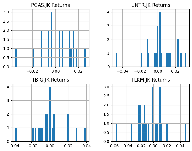
1. Mean & Variance
For this section, for a better illustration of the model, we will randomly generate 4 stocks from the sminfra18 to compose a portfolio to optimize.| date | PGAS.JK | UNTR.JK | TBIG.JK | TLKM.JK |
|---|---|---|---|---|
| 2024-07-10 00:00:00 | 1520.0 | 23550.0 | 1935.0 | 3160.0 |
| 2024-07-11 00:00:00 | 1560.0 | 23500.0 | 1990.0 | 3180.0 |
| 2024-07-12 00:00:00 | 1580.0 | 23500.0 | 2000.0 | 3220.0 |
| 2024-07-15 00:00:00 | 1580.0 | 23750.0 | 1970.0 | 3160.0 |
| 2024-07-16 00:00:00 | 1610.0 | 23800.0 | 2010.0 | 3100.0 |
| date | PGAS.JK Returns | UNTR.JK Returns | TBIG.JK Returns | TLKM.JK Returns |
|---|---|---|---|---|
| 2024-07-11 00:00:00 | 0.026315789473684292 | -0.002123142250530785 | 0.028423772609819098 | 0.006329113924050667 |
| 2024-07-12 00:00:00 | 0.012820512820512775 | 0.0 | 0.005025125628140614 | 0.012578616352201255 |
| 2024-07-15 00:00:00 | 0.0 | 0.010638297872340496 | -0.015000000000000013 | -0.018633540372670843 |
| 2024-07-16 00:00:00 | 0.018987341772152 | 0.002105263157894832 | 0.020304568527918843 | -0.01898734177215189 |
| 2024-07-17 00:00:00 | 0.006211180124223503 | 0.0 | -0.00995024875621886 | 0.048387096774193505 |
2. Monte Carlo Simulation
Monte Carlo simulation is a powerful technique used in portfolio optimization to assess the potential outcomes of different investment strategies or different allocations under varying conditions. It involves generating multiple scenarios based on statistical models and random sampling. Implementing Monte Carlo simulation in Python involves combining statistical analysis, simulation, and optimization techniques to gain insights into portfolio performance under different allocations. For our analysis, we will run a simulation on different allocations of the same stocks to find the optimum allocation. A single run of the simulation is shown in the code below.3. Sharpe Ratio
Sharpe ratio measures the risk-adjusted return by subtracting the risk-free rate. We want the portfolio weight randomly generated by Monte Carlo Simulation with the highest sharp ratio. See more here - link4. Efficient Frontier
The efficient frontier rates portfolios on a coordinate plane. Plotted on the x-axis is the risk, while return is plotted on the y-axis—annualized standard deviation is typically used to measure risk, while compound annual growth rate (CAGR) is used for return. The volatility, return and sharpe ratio values for the simulation are plotted below.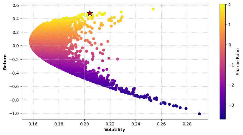
MVO with Scipy Minimized Function
1. Overview on the method
In our next analysis method, we will optimize the same portfolio allocation mathematically using the minimize function in Scipy (a library in Python) and Sharpe ratio. Portfolio optimization using Scipy’s minimize function and the Sharpe ratio involves using mathematical optimization to find the optimal asset allocation that maximizes the Sharpe ratio—a measure of risk-adjusted returns. The basic principle is to find the Sharpe ratio for a random allocation and then multiply it by -1 to make it negative and then minimize it to obtain the allocation weights that gives the highest Sharpe ratio.2. Scipy Minimize Function
- 0.4136 (or 41.36%) is allocated to the first asset.
- 0.5864 (or 58.64%) is allocated to the second asset.
- 0.0000 (or 0%) is allocated to the third asset.
- 1.06e-14 (or essentially 0%) is allocated to the fourth asset.
3. Result Comparison

Summary & Recommendation
Workshop Summary This workshop explored key concepts in portfolio optimization, focusing on sector analysis, stock selection methodologies, and mean-variance optimization (MVO). The main topics included:- Understanding Sectors and Stock Indices: Selecting stock indices based on business objectives and industry trends using SectorsAPI. Data Collection and Exploration: Retrieving stock data from APIs and performing exploratory data analysis (EDA) to identify trends and outliers.
- Stock Selection via Diversification Strategy: Applying EDA and normalization techniques to score companies on growth potential, dividends, and financial indicators.
- Mean-Variance Optimization (MVO): Implementing portfolio optimization through Monte Carlo simulations and the Scipy minimized function to maximize returns for a given risk level.
- Macroeconomic Conditions: Factors like interest rates and inflation can significantly impact stock performance.
- Valuation Metrics: Evaluating P/E ratios, price-to-book, and free cash flow yield is critical for assessing valuations.
- Risk Factors: Systemic and geopolitical risks should be considered.
- Sustainability and ESG Factors: Institutional investors increasingly prioritize environmental, social, and governance criteria for long-term growth.
- Monte Carlo Simulation: This method generates thousands of random portfolios to visualize the efficient frontier and calculate the Sharpe ratio. While flexible, it can be computationally expensive and may not converge on the most efficient portfolios.
- Scipy Minimized Function: This deterministic method computes the optimal portfolio by minimizing volatility or maximizing the Sharpe ratio under specific constraints. It is faster but may be limited by initial guesses for weights and a narrower exploration of possibilities.
- Dynamic Risk Modeling: Adjusting risk models for changing correlations and volatilities.
- Transaction Costs and Liquidity Constraints: Factoring in trading costs and asset liquidity in optimization models.
- Non-Normal Return Distributions: Accounting for tail risk and skewness in return distributions.